In summer semester 2016 I attended the seminar Algorithmic Methods in the Humanities at KIT. My talk was about Latent Dirichlet Allocation. The slides can be found here. The objective of this write-up is to explain what Latent Dirichlet Allocation is by giving a concrete example and to provide some intuition on how it works.

Topics

Topic models are used to discover topics in documents. A topic may be defined as a distribution over words; consider, for instance, the following distribution over words, representing computer science:

0.15*programming, 0.1*algorithm, 0.05*turing machine, 0.05*complexity, 0.05*software,… etc.

Latent Dirichlet Allocation is one instance of a topic model. LDA’s defining feature is the generative process assumption. In machine learning generative models are used to generate data points. Given some data (e.g. a text corpus) in a generative model it is assumed that there exists some process in the background which has generated the data. In the context of topic models, this means that the process selected a topic first and then decided which word to pick from that topic. The generative process has certain parameters and it is assumed that there must be a certain configuration that is most likely to have generated the observation. Now the goal is to infer those hidden parameters. Inference can be seen as reversing the generative process. That means that we want to uncover the most likely configuration that has produced a document. In the case of Latent Dirichlet Allocation the hidden variables are the per-document topic distribution, the per-document per-word topic assignments and the topics themselves.

Generative Process Pseudocode:
In Number of words \(N\), Number of topics \(K\), Dirichlet parameters \(\alpha \in \mathbb{R}_{> 0}^K, \beta \in \mathbb{R}_{> 0}^N\)
Out \(D\) documents (bag-of-words) with \(N\) words each
— Choose \(\theta_d \, \sim \, \mathrm{Dir}(\alpha)\)
— Choose \(\varphi_k \, \sim \, \mathrm{Dir}(\beta)\)
—For each word position \(d,n\)
—— Choose a topic \(z_{d,n} \,\sim\, \mathrm{Multinomial}(\theta_d).\)
—— Choose a word \(w_{d,n} \,\sim\, \mathrm{Multinomial}( \varphi_{z_{d,n}})\)

where \(d \in \{1,...,D\}\) and \(n \in \{1,...,N\}\).

\(\theta_d\), the topic distribution, and \(\varphi_k\), the distribution of words for topic \(k\), are distributed according to the so called Dirichlet distribution. A discussion about this distribution and its properties is omitted here, since it would only be of little help to gain insight.

The idea of the following code is simple: Wikipedia articles from three topics, namely computer science, philosophy and linguistics are put in one corpus. The second step is to let LDA reconstruct those three topics. (The complete notebook can be found here.)

The example makes use of gensim, a topic modelling library.

%matplotlib inline
import matplotlib.pyplot as plt
import numpy as np
import pandas as pd
from gensim import corpora
from gensim.utils import simple_preprocess
from gensim.models import ldamodel
from gensim.parsing.preprocessing import STOPWORDS
import wikipedia

First, scrape some Wikipedia articles.

computer_science = ["Algorithm", "Computation", "Computer Programming", 
                    "Programming Language","Computational complexity theory",
                    "Computability theory", "Artificial Intelligence"]

philosophy = ["Epistemology", "Metaphysics", "Continental philosophy" 
              "Ancient Greek", "Ethics", "Aesthetics", 
              "Art", "Phenomenology (philosophy)", "Pythagoras", "Plato"]

linguistics = ["Language" ,"Semantics", "Syntax", "Phonology", "Grammar",
               "Phonetics", "Pragmatics",  "Corpus linguistics", 
               "Linguistic prescription", "Linguistic description"]
articles = computer_science + philosophy + linguistics
documents = [wikipedia.page(title).content for title in articles]

The following functions are used for preprocessing; the texts are tokenized and STOPWORDS, like of, the, and, or, this, that, over,… are removed, as they don’t convey much information.

def tokenize(text):
    return [token for token in simple_preprocess(text) if token not in STOPWORDS]

def preprocessing(documents):
    # see:  https://radimrehurek.com/gensim/tut1.html  
    # remove common words and tokenize
    texts = [[word for word in document.lower().split() if word not in STOPWORDS and 
              word not in special_chars] 
             for document in documents]

    # remove words that appear only once
    all_tokens = sum(texts, [])
    tokens_once = set(word for word in set(all_tokens) if all_tokens.count(word) == 1)
    texts = [[word for word in text if word not in tokens_once] for text in texts]

    dictionary = corpora.Dictionary(texts)
    preprocessed_docs = [dictionary.doc2bow(text) for text in texts]  # bow = bag of words
    return preprocessed_docs, dictionary

CORPUS, dictionary = preprocessing(documents)

The number of topics has to be chosen a priori. One can think of LDA as a clustering algorithm. Like K-Means, LDA needs the number of ‘clusters’ (i.e. topics) it is supposed to find in the data.

K = 3 # number of topics
lda = ldamodel.LdaModel(CORPUS, id2word=dictionary, 
                        num_topics=K, update_every=1, 
                        chunksize=1, passes=350)
corpus_lda = lda[CORPUS]
for i in range(K):
    print "TOPIC " + str(i+1) + ":   "+ lda.print_topic(i) + "\n"

LDA produces the following three topics and seems to correctly reproduce the three clusters. Notice that, according to our dataset, the most important word for topic 1 is programming. This word defines the topic to a proportion of only ~1%.

Only the most prevalent words are listed in the following

    TOPIC 1:   0.010*programming + 0.009*turing + 0.008*problem + 0.007*machine + 0.006*problems +
        0.006*algorithms + 0.006*algorithm + 0.006*set + 0.006*complexity + 0.005*time

    TOPIC 2:   0.008*plato + 0.006*plato´s + 0.006*knowledge + 0.005*pythagoras + 0.005*philosophy + 
0.004*phenomenology + 0.004*greek + 0.004*according + 0.004*socrates + 0.003*theory

    TOPIC 3:   0.019*language + 0.009*languages + 0.007*art + 0.005*meaning + 0.005*linguistic + 
        0.005*human + 0.004*ethics + 0.004*speech + 0.004*study + 0.004*grammar

We now have a trained model and can query a new instance. This means, that we can use the model to calculate how an unseen document, (i.e. a document that has not been used to train the model) is composed of the previously determined topics.

noam = wikipedia.page("Noam Chomsky").content

bow_vector = dictionary.doc2bow(tokenize(noam))
print lda[bow_vector]

    [(0, 0.032599745516170064), (1, 0.30504589551791855), (2, 0.66235435896591133)]

The 0.66235435896591133 inside the last tuple means that the Wikipedia article on Noam Chomsky is to ~66.24% about linguistics. Since Naom Chomsky is primarily a linguist, LDA satisfies our expectation.

# code used to plot the bar graph below
def topic_distribution(lda_corpus_model):
    data = {}
    for i, dist in enumerate(lda_corpus_model):
        distribution = np.array([0.01,0.01,0.01])
        for topic_weight in dist:
            distribution[topic_weight[0]] = topic_weight[1]
        data.update({articles[i]: distribution})
    return data
        

data = topic_distribution(list(lda[CORPUS]))

n = 20
df2 = pd.DataFrame(np.array(data.values())[:n], columns=["CompSci", "Philo", "Ling"], 
                   index=data.keys()[:n])
df2.plot.bar(figsize=(15,8), fontsize=15);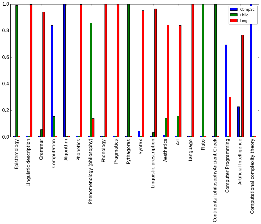

Figure 1: Topic proportions for some of the Wikipedia articles that were used to train the model. The Wikipedia article on ‘Pythagoras’, for instance, is classified as a document in the category ‘philosophy’ with very high confidence. Note that albeit the confidence is very high it is not 100%. Due to the model every document exhibits all the K topics, but to a very different degree.

LDA can also be viewed from a dimensionality reduction perspective:

It performs dimensionality reduction, relating each document to a position in low-dimensional "topic" space. In this sense, it is analogous to PCA, except that it is explicitly designed for and works on discrete data. ¹

How it works

The goal is to infer hidden or latent variables (topics) from observed ones (words). We call the \(nth\) word from the \(dth\) document \(w_{d,n}\). Remember that we assumed that all \(w_{d,n}\) come from a generative process/model. This generative model defines several dependencies, which can be depicted with plate notation. This notation is a concise method for visualizing the factorization of the joint probability. A shaded node means that a random variable is observed.

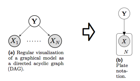
Figure 2: Plate notation as a way to summarize conditional dependencies

The joint probability of the probabilistic graphical model depicted above is

Latent Dirichlet Allocation is a hierarchical Bayesian model. With plate notation there’s a concise way to represent the hierarchical structure. Be aware of the nested structure - the \(D\) plate contains the \(N\) plate, which means that the topic assignments \(z_{d,n}\) and the corresponding words \(w_{d,n}\) would be repeated \(N \times D\) times, if the plate notation was “unfolded”.

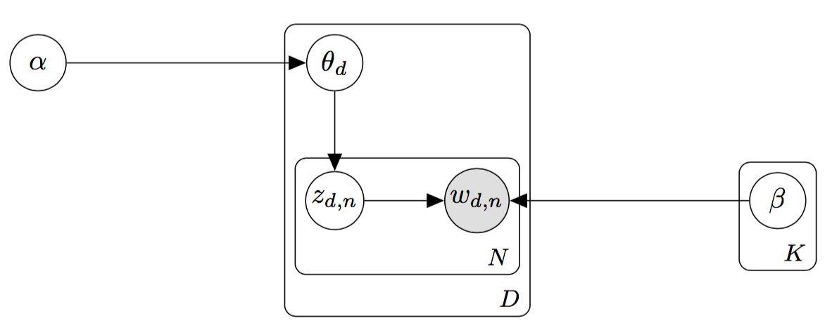
Figure 3: LDA represented in plate notation

In order to get the topics and the assignment of a word \(w_{d,n}\) to a certain topic (\(z_{d,n}\)), the inferential problem must be solved. This means, that we use the conditional dependencies to compute the posterior of the latent variables. With Bayes’ theorem:

However, as it turns out, this is intractable to compute, which is quite common for posterior distributions and is due to the fact that a solution to the denominator of the above equation would involve integrating over all possible hidden topic structures ².

One solution to this problem is called Gibbs sampling. Sampling is a way to approximate a solution when exact computation is infeasible. Let \(m_{d,k}\) denote the number of words that are assigned to topic \(k\) in document \(d\) and \(m_{k,w}\) the number of times \(w\) is assigned to topic \(k\) over the whole corpus. First every word \(w_{n,d}\) is randomly assined to one of the \(K\) topics. Then, in each iteration Gibbs sampling samples a word and reassigns it to one of the \(K\) clusters. This decision is made by evaluating the probability of the word belonging to the cluster \(c_i, \; i \in \{1,...,K\}\). The probability is defined to be the product of the number of words that are assigned to topic \(k\) in the document and the the number of times the sampled word \(w\) was assigned to topic \(k\) over the corpus:

The equation ensures that words from the same document have higher probability of being assingned to the same topic.

Example Let’s say there are ten documents with 1000 words each and the word Pythagoras occurs 20 times across those documents. We chose \(K=3\). In the initialization step this word was randomly assigned ten times to topic 1, six times to topic 2 and four times to topic 3.

Now we consider one of the 10 documents \(d\) and we assume that the topic distribution of \(\theta_d\) is approximately uniform, meaning that ~333 words were assigned to topic 1, topic 2 and topic 3. Now, if the Gibbs sampler comes across the word Pythagoras it will most likely (re)assign it to topic 1. The counts are updated: if Pythagoras was previously assigned to topic 2, then the word counts would look like this:

Table 1: Word distribution (counts) after assigning Pythagoras to topic 1. \(m_{k,w}\) is the number of words assigned to topic k in doc d.

This procedure of (re)assigning words is repeated several times. Gibbs sampling will eventually converge, yielding a topic assingment for every word in the corpus. From those one can compute the topic distribution \(\theta_d\) for each document and the word distribution \(\varphi_k\) for each topic.

Conclusion

Topic models are a tool to find the hidden topic structure in large text corpora. The hidden structure must be uncovered in order to gain information about the low-dimensional structure behind a text corpus. A topic modeling algorithm takes a corpus as an input and will output the topics running through that corpus. The generative process is the essential idea behind Latent Dirichlet Allocation. Reversing the generative model (identifying hyperparameters) by applying Gibbs sampling yields a solution of the inference problem.

References

• Blei, David M., Andrew Y. Ng, and Michael I. Jordan. “Latent dirichlet allocation.” Journal of machine Learning research 3.Jan (2003): 993-1022.

• Darling, William M. “A theoretical and practical implementation tutorial on topic modeling and gibbs sampling.” Proceedings of the 49th annual meeting of the association for computational linguistics: Human language technologies. 2011.

• Griffiths, Thomas L., and Mark Steyvers. “Finding scientific topics.” Proceedings of the National academy of Sciences 101.suppl 1 (2004): 5228-5235.

Further Reading/Watching

• Blog post: Introduction to Latent Dirichlet Allocation (by Edwin Chen)
• There’s an excellent lecture on Latent Dirichlet Allocation by David Blei: Machine Learning Summer School (MLSS), Cambridge 2009

Footnotes